People You May Konw

Problem Statement

People You May Know (PYMK) is a list of users with whom you may want to connect based on things you have in common, such as a mutual friend, school, or workplace.

Clarifications or Assumptions

1. What’s the objective/motivation?
   • May I assume the motivation of the PYMK feature is to help users discover potential connections and grow their network?
2. How to define ‘connections’?
   • May I assume that people are friends only if each is a friend of the other?
3. What should I consider for forming connections?
   • To recommend potential connections, a huge list of factors must be considered, such as educational background, work experiences, existing connections, historical activities. Should I focus on the most important factors?
4. Define the scale
   • How many connections does an average user have? (like 1000)
   • What’s the total number of users on this platform? (like 1 billion)
   • How many of them are daily active users? (like 300 million)
5. Model Dynamics
   • May I assume that the social graph of most users are not dynamic, meaning that their connections don’t change significantly over a short period.

Frame as an ML Business Objective

Business Objective

The motivation for building the system is to enable users to discover new connections more easily and grow their networks.

Success is measured by increased user engagement with the network (connection requests sent and accepted)

ML Objective

• Maximize the number of formed connections between users (link prediction or ranking problem), The ultimate metric is how many recommended connections actually convert into real connections
• Define the input and the output
  • input: a user
  • output: a list of users

Choosing ML methology

There are commonly two approaches for PYMK: Pointwise Learning-To-Rank (LTR) and Edge Prediction.

1. Pointwise LTR

• Why this approach:
  • The pointwise LTR transforms a ranking problem to a supervised learning problem, where the model takes user and a candidate connection pair as inputs, and outputs a score or probability.
  • In cold-start scenarios where rich interaction data is lacking, the pointwise LTR can quickly model the similarity between user pairs.
• Why not this approach:
  • This ignores some social context, the inputs are distinct users

2. Edge Prediction

• The entire social context can be represented as a graph, where each node represents a user, and an edge between two nodes indicates a formed connection between two users.
• Use the entire graph as input, and predict the probability of an edge existing between user A and other users

Data Preparation

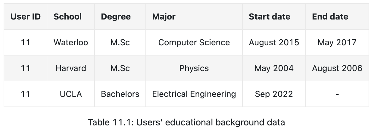
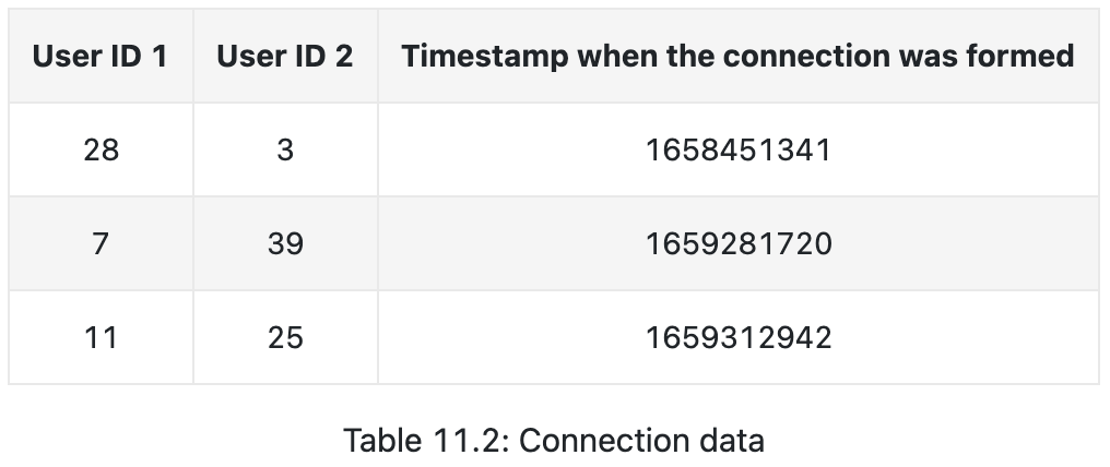
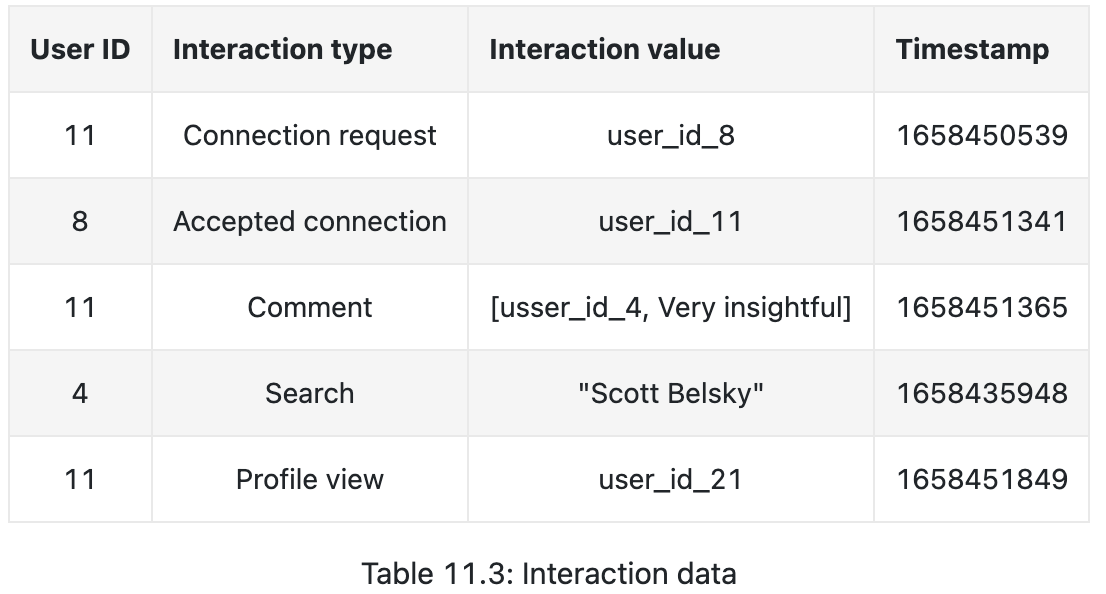
We typically use three types of raw data:

• User
  • demographic data
  • educational and work backgrounds, skills
  • interests
• Connections
  • user pairs (timestamp when connection was formed)
• Interactions
  • connection request, acceptance, comment, search, profile view, etc.

One challenge with this type of raw data is that a specific attribute can be represented in different forms. It is necessary to standarize the raw data.

Feature Engineering

• User Features
  • Demographics: age, gender, city, country, etc.
  • The numbers of connections, followers, following, and pending requests
  • Account’s age
  • The number of received reactions
• User-user affinities
  • Education and work affinity
• Social affinity
  • mutual connections
  • Time discounted mutual connections
  • profile views

Modeling

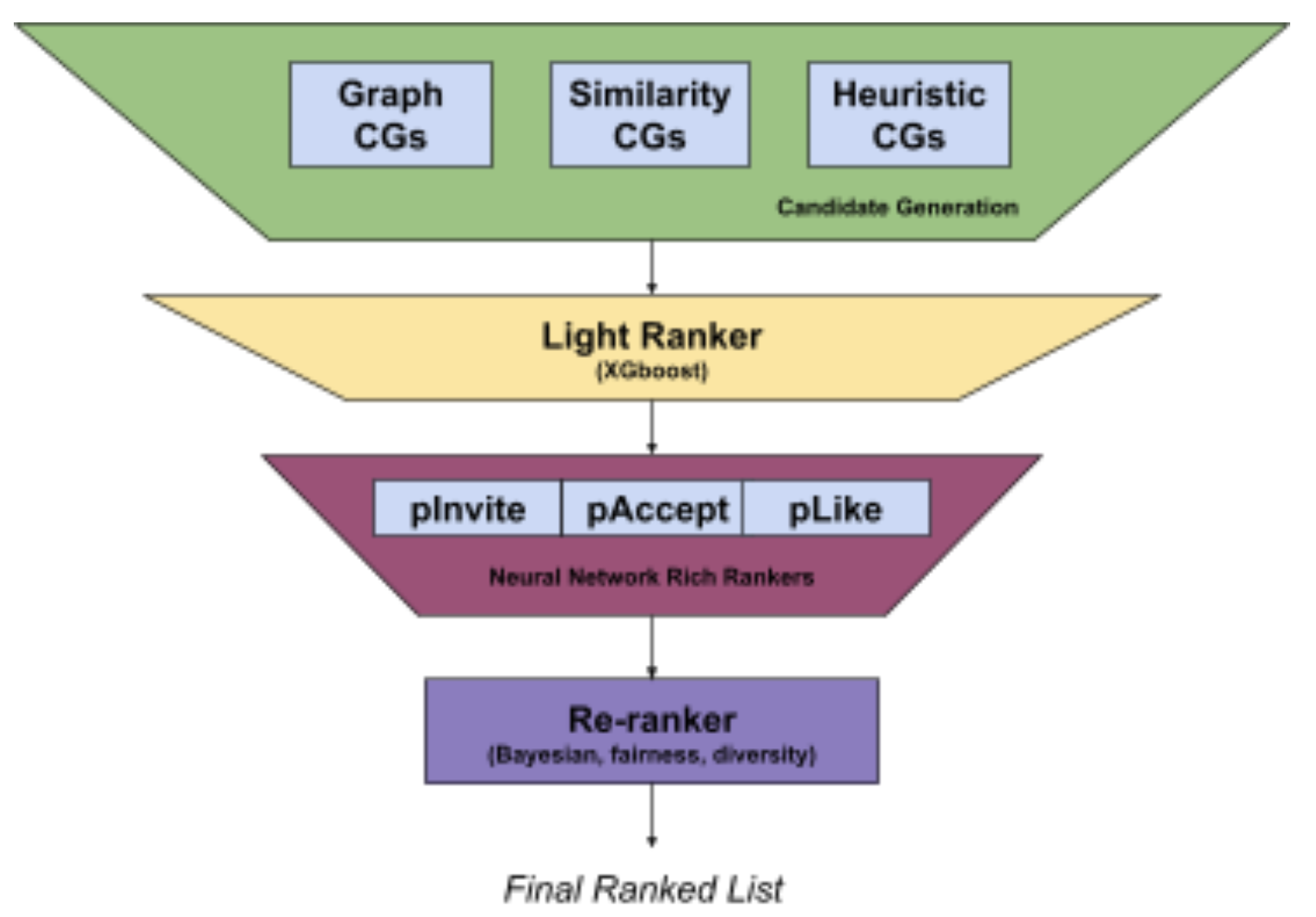
Candidate generation

It consists of multiple retrieval techniques which can be broadly organized into three categories:

• graph-based (graph walk)
  • N-hop Neighbors (N≠1)
    • N is restricted to 3 to control the volume of generated candidates
    • similarity over GNN embeddings should be able to generate N-hop candidates
  • Personalized PageRank (PPR), to run deeper graph walks
    • PPR scores are generated for all (viewer, member) tuples
• similarity-based
  • Embedding Based Retrieval (EBR), standard NN search
  • Two-tower NN
• heuristics-based
  • generated by simple rules (also called filters)

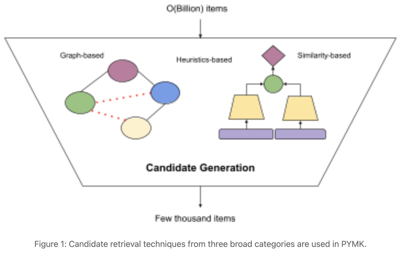
Noted: GNNs actually suffered from the problem of graph isomorphism. Hence, we nowadays rely on explicitly running the N-hop and PPR graph walks to generate candidates.

Light ranker

• Logistic regression
• XGBoost

Heavy ranker

• Deep neural networks

Re-ranker

• ensure fairness, to avoid outcomes like overrepresenting platform power users.
• employ Bayesian Optimization to estimate the most important parameters

Evaluation

Offline metrics:

• Recall@k at CG stage/light ranker
• AUC/Precision@k at heavy ranker
• log-likelihood and diversity metrics at re-ranker

Online metrics:

• A/B tests
  • The total number of connection requests sent in the last X days
  • The total number of connection requests accepted in the last X days

Offline metrics rarely match the online performance measures

• Presentation biases (missing profile photo, laggy UI, position bias, etc.).
• Unintentional errors in deploying models to production.
• Discrepancy between the distribution of offline training data and online data.

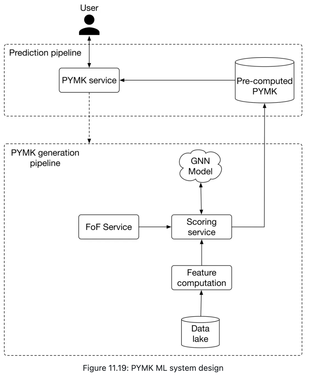
Serving

Online v.s. Batch:

• Online: perhaps takes a long time to make predictions
• Batch: pre-compute potential connections for all users
  • probably end up with unnecessary computations
  • the social graph does not evolve quickly
  • if we want to optimize more, pre-computing PYMK only for active users.

Appendix

Graph-based

In general, a graph represents relations(edges) between a collection of entities(nodes). Graphs can store structural data, there are three general types of prediction tasks that can be performed on structured data represented by graphs:

• Graph-level
  • like chemical compound
• Edge-level
  • like PYMK on social media
• Node-level
  • like predicting whether a person is a spammer or not, given a social network graph

References ⭐

• Building a Large-Scale Recommendation System: People You May Know
• Candidate Generation in a Large Scale Graph Recommendation System: People You May Know