Intro to DenseNet

Abstract

DenseNet is detached from the stereotypical thinking of deepening the number of network layers (ResNet) and widening the network structure (Inception) to improve the performance of the network.

The Limitations

DenseNet and other related networks all share a key characteristic: they create short path from early layers to later layers. There exists some limitations from its pioneering works.

• ResNet combines features through summation (additive identity transformations).
• Stochastic depth improves the training of deep residual networks by dropping layers randomly during training.
  • This makes the state of ResNets similar to (unrolled) RNN.
    The major difference between DenseNet and related works is to use concatenating features-maps.

Advantages

• Improve flow of information and gradients through the network
  • Mitigate the gradient vanishing problem
• Fewer parameters
  • No need to relearn redundant feature-maps
  • DenseNet layer explicitly differentiates between new information and preserved information
  • Each layer is very narrow (e.g., 12 filters per layer)
• Regularizing effect to reduce overfitting

Network	Advantage	Disadvantage
Summation (ResNet)	Parameter Efficiency Improved Gradient Flow Identity Shortcut	Feature Mixing Capacity Limitation
Concatenation (DenseNet)	Feature Preservation Enhanced Feature Propagation Flexibility	Increased Computational Cost Memory-intensive

Structure

In a summary, whereas traditional convolutional networks with $L$ layers have $L$ connections, the densenet network has $\frac{L(L+1)}{2}$ direct connections.
Our basic dense connectivity can be represented as:
$$ x_l = H_l([x_0, x_1, …., x_{l-1}])$$

• Dense Block: To facilitate down-sampling within the architecture and to address concatenation issues arising from changes in the sizes of feature-maps between two blocks.

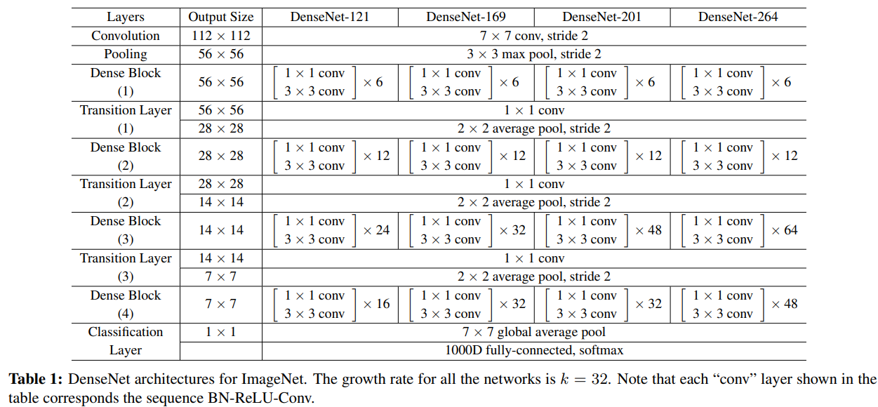
• Composite function: $H_l(.)$ consists of three consecutive operations: batch normalization, ReLU, and a $3\times3$ convolution.

  • The conv layer shown above corresponds the sequence BN-ReLU-Conv.

• Transition Layer: it does convolution and pooling.

• Bottleneck layers: a $1\times1$ convolution can be introduced as bottleneck layer before each $3\times3$ convolution to reduce the number of input feature-maps and to improve computational efficiency.

  • DenseNet-B: BN-ReLU-Conv($1\times1$)-BN-ReLU-Conv($3\times3$)

• Parameters:

  • There is a general trend that DenseNets perform better as $L$ and $k$ increase without compression or bottleneck layers.
  • Growth Rate: The growth rate $k$ regulates how much new information each layer contributes to the global state.
  • Compression: $0<\theta<1$ is referred to as the compression factor. It is set to 0.5 to improve model compactness which is to reduce the number of feature-maps at transition layer.
    • DenseNet-BC: both the bottleneck and transition layers with $\theta<1$ are used.

The following heatmaps shows the average absolute weight to serve as a surrogate for the dependency of a convolution layer on its preceeding layer.

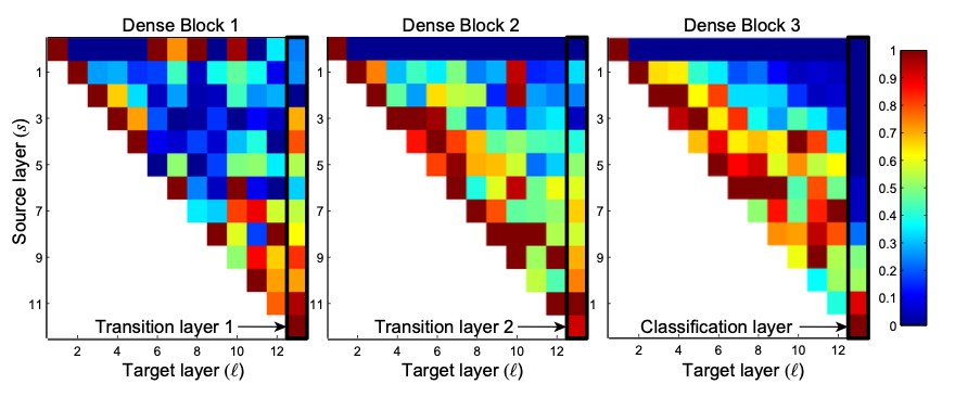
• The top row of each heatmap indicates that the transition layer outputs many redundant features.
• The right-most column shows that the weights of the transition layer also spread their weight across all layers within the preceding dense block.
  • The DenseNet-BC helps to alleviate this problem.
• The column shown on the very right suggests that there may be some more high-level features produced late in the network.

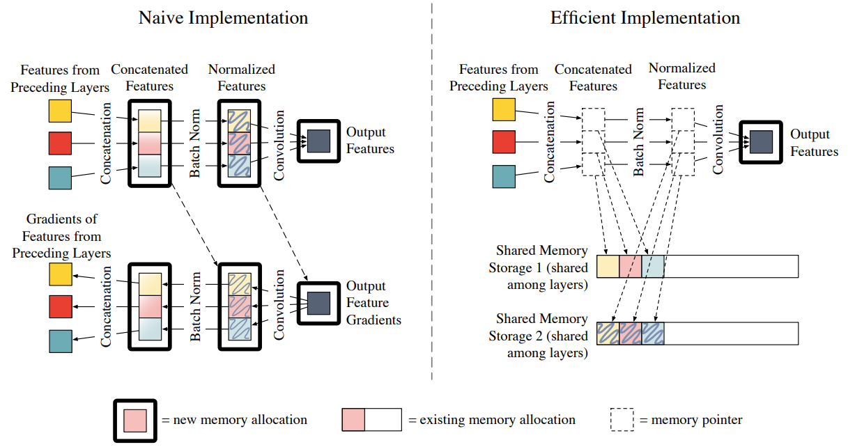
Memory-efficient Implementation

References ⭐

• Densely Connected Convolutional Networks