Recommendation System

Problem Statement

Display media recommendations for a specific user. Type of user feedback includes explicit and implicit feedbacks. The implicit feedback allows collecting a large amount of training data.

Metrics

• Online metrics
  • Engagement rate
  • Videos watched
  • Session watch time (better than the above intuitively)
• Offline metrics
  • mAP (Mean Average Precision) @ N (length of the recommendation list)
    • $P = \frac{num_of_relevant_recommendations}{total_num_of_recommendations}$
    • $P @k = $proportion of all examples above that rank which are from the positive class. Precision represented at each cut off k.
    • $AP@N = \frac{1}{m}\sum_{k=1}^{N}P(k)*rel(k)$ where the $P(k)$ only contributes to $AP$ (average precision) if the recommendation at position $k$ is relevant.
  • mAR (Mean Average Recall) @ N
    • mAR @ N at a high-level, showes how well the recommender recalls all the items with positive feedback.
    • $r = \frac{num_of_relevant_recommendations}{num_of_all_possible_relevant_items}$
  • F1 Score
    • $F1 score = 2 * \frac{mAR*mAP}{mAP+mAR}$
  • For optimizing ratings
    • Optimize the recommendation system for getting the ratings (explicit feedback).
    • $RMSE = \sqrt{\frac{1}{N}\sum_{i=1}^N(\hat{y_i} - y_i)^2}$

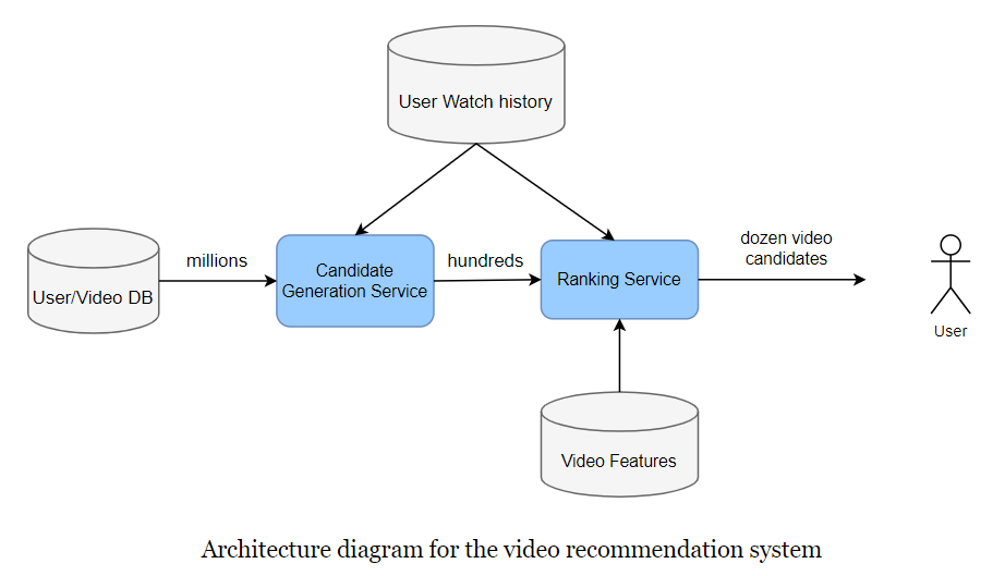
Architecture

There are two stages, candidate generation, and ranking. The reason for two stages is to make the system scale.

Candidate Generation

This component focuses on higher recall.

• Collaborative filtering

  • Nearest Neighborhood
    • Collaborate with similar users to generate candidate media for active user.
    • Caveat:
      • This process will be computationally expensive.
      • This sparsity of this matrix poses the cold start problem (New users ans movies).
  • Matrix factorization
    • Latent vectors (User profile matrix - $nM$, Media profile matrix - $Mm$) can be thought of as features of a movie or a user.
  • It does not require domain knowledge to create profiles, thus, this filtering suffers from the cold start problem.

• Content-based filtering

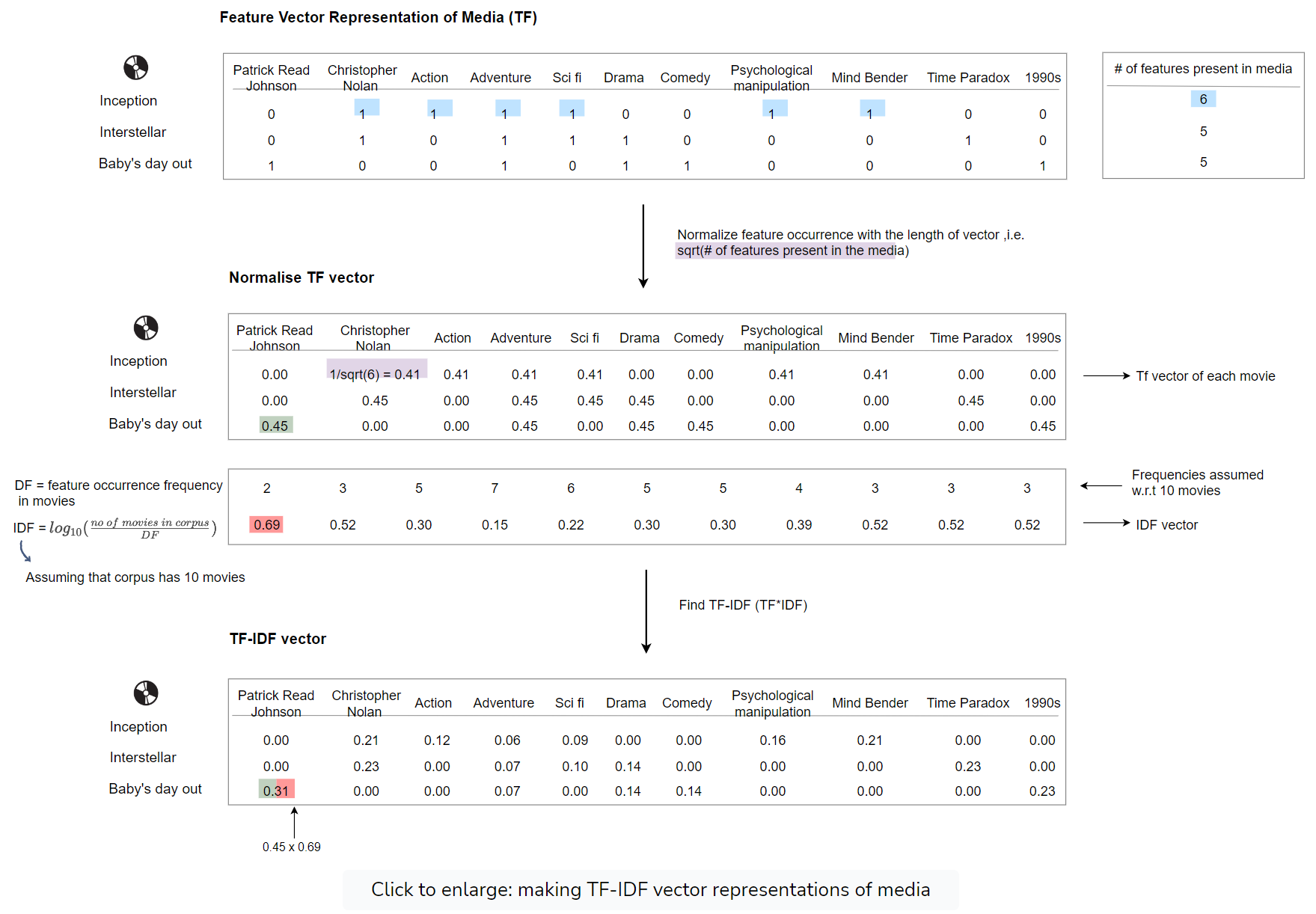
  • Make recommendations based on the characteristics or attributes of the media the users have already interacted with.
  • Represent the media as vectors containing the TF of all the attributes; Normalize the TF by the length of the vectors; Multiply normed TF and IDF element-wise to make TF-IDF vectors.
    • Similarity with historical interactions
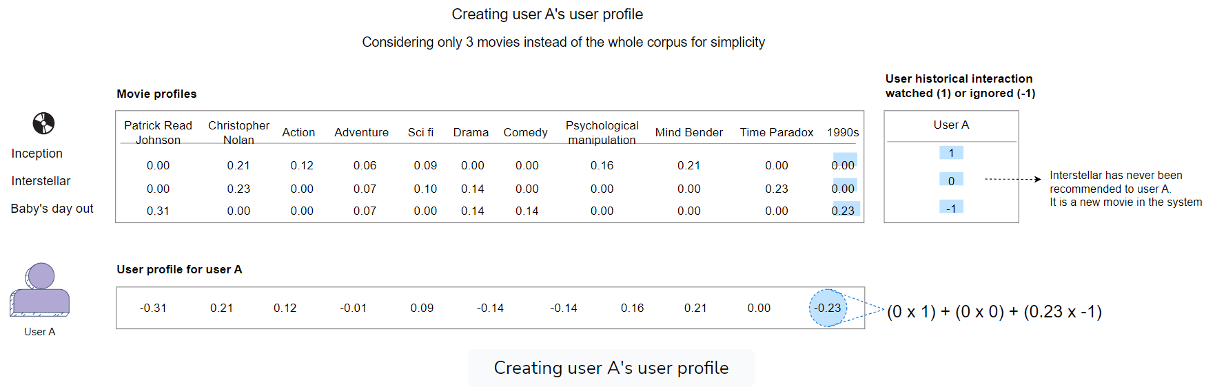
    • Similarity between media and user profiles
      • The user profiles can be built from historical interactions with media.
  • It requires some initial input from the user regarding their preferences.

• Embedding-based similarity
  • The NNs allow us to use all the sparse and dense features.
  • Set up a two-tower model with one tower feeding in media only sparse and dense features and the other tower feeding in user-only sparse and dense features.
  • Loss function: $min(abs(dot(u, m) - label))$
  • The NN technique suffers from the cold start problem.

Training Data Generation

• Generating training samples
  • The data will be split as positive, negative, ot falls into the uncertainty bucket (watch time falls between 20%-80%).
• Balancing samples by randomly downsampling negative examples.
• Weighting training examples based on watch time or other features.
  - One caveat of utilizing weights is that the model might only recommend content with a longer watch time.
• Train test split: models should be built with the intent to forecast the future.

Ranker

This component focuses on higher precision.

• Logistic regression or random forest

  • Reasons
    • Training data is limited.
    • You have limited training and model evaluation capacity.
    • Model explainability is required.
    • An initial baseline is required.

• Deep NN with sparse and dense features

  • Reasons
    • Hundreds of millions of training examples and capacity should be available.
    • Model interpretability is not required.
  • Important sparse features
    • Videos that the user has previously watched
    • The user’s search terms
    • The sparse features are list-wise (Averaged pooling before being fed to network).

• Re-ranking: bringing diversity or past watches to the recommendation.

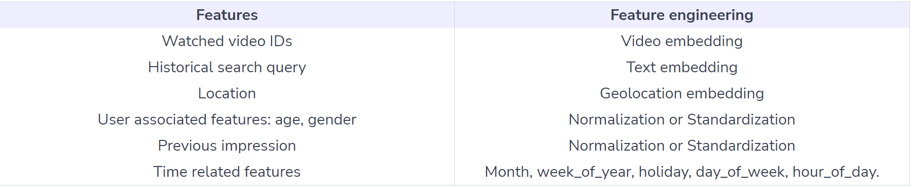
Feature Engineering

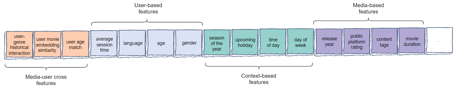
• User-based features
• Context-based features
• Media-based features
• Media-user cross features

Example: Video Recommendation

Problem statement:

Build a video recommendation system for YouTube users. Recommendation Youtube is extremely challenging from following major perspectives:

• Scale: it is required to handle YouTube’s massive user base and corpus;
  • Highly specialized distributed learning algorithms
  • Efficient serving systems
• Freshness: Balancing new content with well-established videos;
• Noise: Historical user behavior is inherently difficult to predict because:
  • Sparsity and a variety of unobservable external factors
  • Metadata associated with content is poorly structured

Requirements

Type	Desired requirements
Training	High throughput with the ability to retrain many times per day
Inference	Latency from 100ms to 200ms Balances between exploration vs. exploitation

Metrics:

Offline: Precision, recall, ranking loss, and logloss;
Online: A/B testing via live experiments to compare Click Through Rates, watch time and Conversion rates.

Model

Candidate Generation
Neural network model is used to mimick matrix factorization. A key advantage of that is that arbitrary continuous and categorical features can be easily added to the model. Therefore, our approach can be viewed as a non-linear generalization of factorization techniques.

The recommendation problem can be posed as extreme multiclass classification where the prediction problem becomes accurately classifying a specific video watch time $w_{t}$ at time $t$ among millions of videos $i$ (classes) from a corpus $V$ based on a user $U$ and context $C$.
$$P(w_t=i|U,C) = \frac{e^{v_iu}}{\sum_{j\in V}{e^{v_ju}}}$$

We use the implicit feedback of the watches to train the model (where a user completing a video is a positive example), where explicit feedback (thumbs up/down, in-product surveys, etc) is extremely sparse;

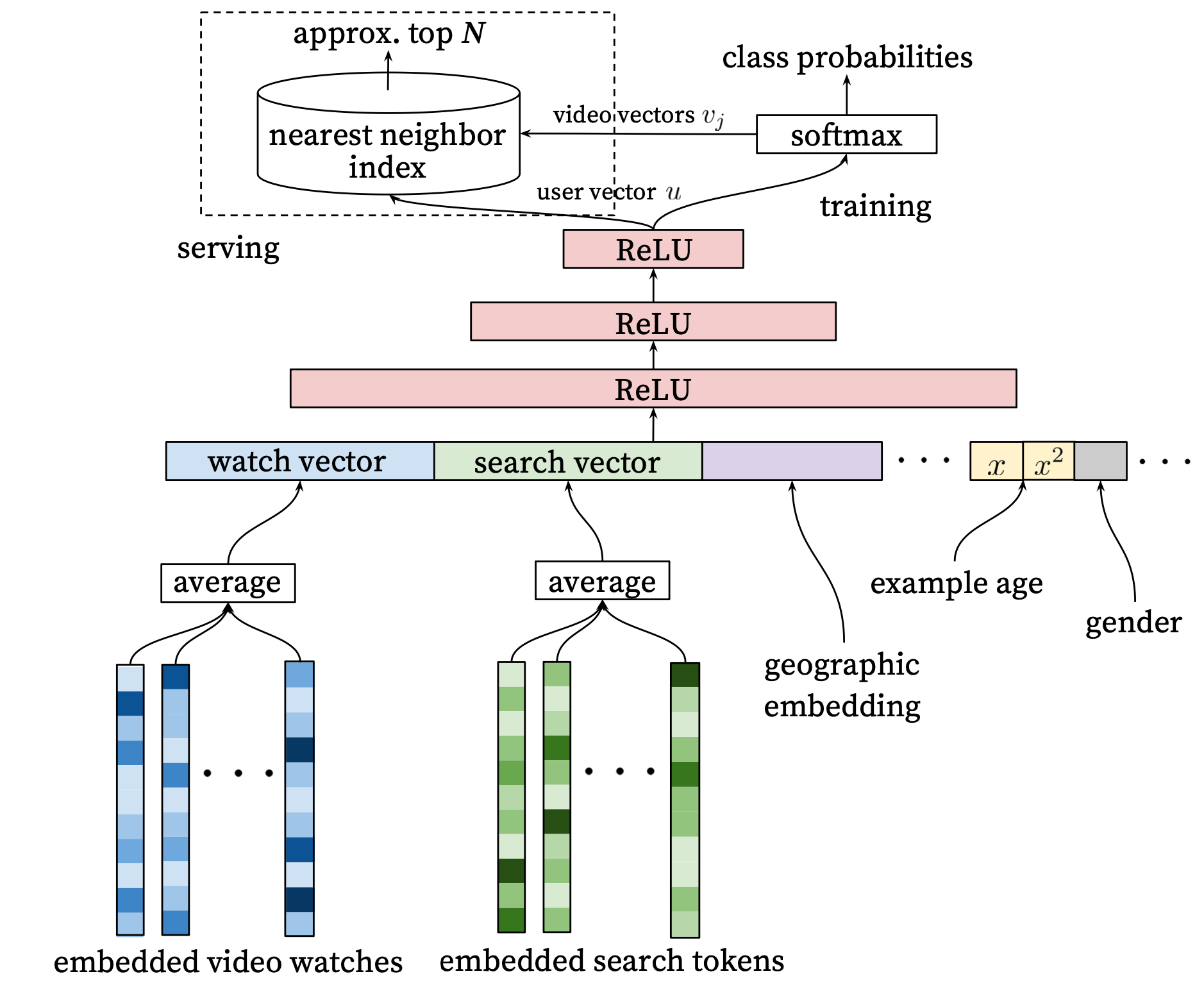
Personally speaking, the diagram might intuitively suggest that video embedding vectors are “outputs” from the softmax layer. However, the pre-learned video embedding vectors are used to calculate their similarity with the user vector through the softmax layer. The final recommendation list is then quickly determined through nearest neighbor search or other efficient methods.

• Efficient Extreme Multiclass
  Scoring millions of items under a strict serving latency of tens of milliseconds requires an approximate scoring scheme sublinear in the number of classes.

  • Traditional softmax needs speeding up
  • Hierarchical softmax is not able to achieve comparable accuracy
  • Scoring problem reduces to a nearest neighbor search; A/B results were not particularly sensitive to the choice of nearest neighbor search algorithm.

• Embedding
  Each query is tokenized into unigrams and bigrams and each token is embedded and normalized.

High dimensional embeddings for each video in a fixed vocabulary. The network requires fixed-size dense inputs and performs several strategies on concatenated features (embedding).

• Heterogeneous Signals
  Machine learning systems often exhibit an implicit bias towards the past.
  Video popularity is highly non-stationary but the multinomial. To correct for this, we feed the age of the training example as a feature during training. At serving time, this feature is set to zero (or slightly negative).

• Label and Context Selection
  We need to take care of the strategy for selecting training examples.

  • Training examples are generated from all Youtube watches to avoid overly exploitation;
  • Generate a fixed number of training examples per user, effectively weighting our users equally in the loss function. In order to prevent a small cohort of highly active users from dominating the loss.

• Surrogate problem
  Recommendation often involves solving a surrogate problem and transferring the result to a particular context. Sometimes the choice of surrogate problem is difficult to measure with offline experiments or compute directly.

• Withhold information from the classifier
  Prevent the model from exploiting the structure of the site and overfitting the surrogate problem, by discarding sequence information and representing search queries with an unordered bag of tokens.

• Asymmetric consumption patterns
  In order to not leak future information and not ignore any asymmetric consumption patterns.

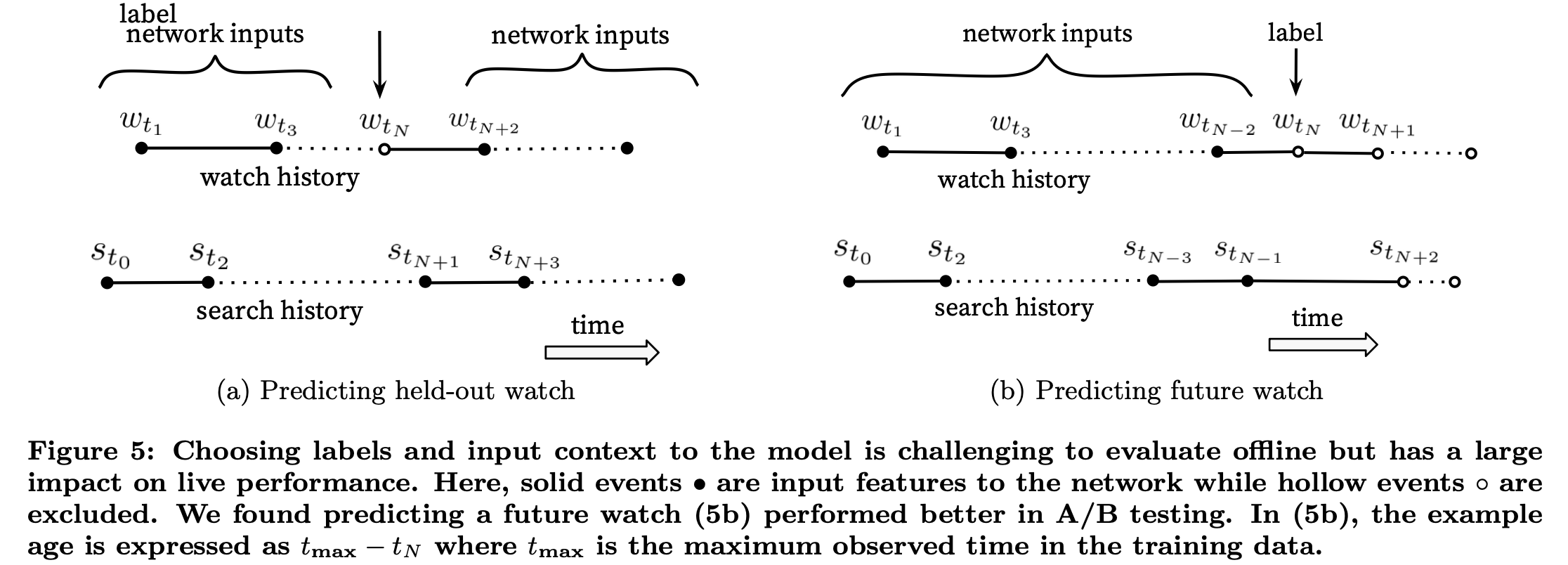
We rollback a user’s history by choosing a random watch and only input actions the user took before the held-out label watch.

Ranking
Our features are segregated with traditional taxonomy of categorical and continuous/ordinal features.

• Features are further split into “univalent” or “multivalent”;
  • “univalent”: contribute to a single value
  • “multivalent”: contribute to a set of values
• Features are further split into “impression” or “query”;
  • “impression”: properties of the item, being computed for each item scored;
  • “query”: properties of the user/context, being computed for once per request;

Feature Engineering
The main challenge is in representing a temporal sequence of user actions and how these actions relate to the video impression being scored.

• The most important signals are those that describe a user’s previous interaction with the item itself and other similar items;
• Propagate information from candidate generation into ranking models;
• Introducing “churn” in recommendations (successive requests do not return identical lists), by including features describing the frequency of past video impressions;

Embedding Categorical Features
Very large cardinality ID spaces:

• Been truncated by including only the top $N$ after sorting based on their frequency in clicked impressions;
• Out-of-vocabulary values are simply mapped to the zero embedding;
• Multivalent categorical feature embeddings are averaged before being fed;

Categorical features in the same ID space share underlying embeddings:

• Sharing embeddings is important for improving generalization, speeding up training and reducing memory requirements.
• The overwhelming majority of model parameters are in these high-cardinality embedding spaces;

Normalizing Continuous Features
Neural networks are notoriously sensitive to the scaling and distribution of their inputs.

• Raw normalized features
  • The continuous feature $x$ with distribution $f$ is transformed into $\overline{x}$ by scaling the values such that the feature is equally distributed in $[0,1)$, using cumulative distribution (CDF) $\overline{x} = \int^{x}_{-\infty}{df}$.
  • The integral is approximated with linear interpolation.
• Super- and sub-linear forms ($\overline{x}^{2}$ and $\sqrt{\overline{x}}$) of features
  • Giving the network more expressive power;
  • Input powers $\overline{x}^{2}$ is found to improve offline accuracy;

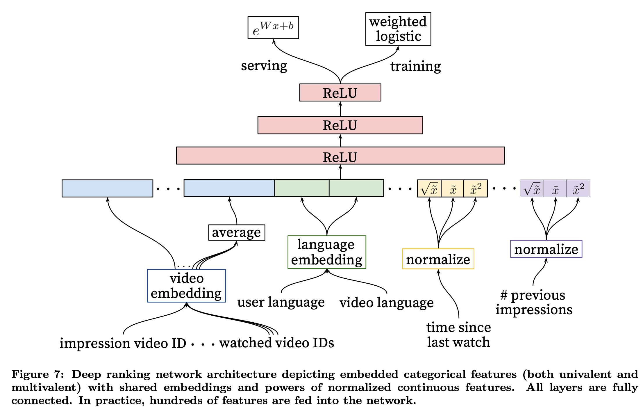
Modeling Expected Watch Time
Weighted logistic regression;

• Positive (clicked) impressions are weighted by the ovserved watch time on the video;
• Negative (unclicked) impressions all receive unit weight;
  Odds learned by the logistic regression is
  $$\frac{\sum{T_i}}{N - k}$$
• $N$ is the number of training examples
• $k$ is the number of positive impressions
• $T_i$ is the watch time of the $i$th impression
  The learned odds are approximately $E[T](1 + P)$
• $P$ is the click probability, and $E[T]$ is the expected watch time of the impression
• For inference, the exponential function $e^{x}$ is used as the final activation function to produce these odds that closely estimate expected watch time.
  • Non-negative outputs
  • Adjustable range
  • Non-linear Transformation of linear relationships
  • Approximating probability products
    • When predictions are close to 0, where $e^{x}$ approximates $1+x$, echoing the earlier mentioned approximation relation $E[T](1 + P)$;
• The intuitive explanation of this formula is:
  • When there is no click, the watch time is likely to be close to the baseline expected watch time $E[T]$;
  • When there is a click, the watch time may increase, and this increase is proportional to the click probability $P$;

Calculation&&Estimation

• Assumptions:
  • Video views are $150$ billion per month
  • $10%$ of videos watched are from recommendations (a total of $15$ billion)
• Data Size:
  • Each feature row takes $500$ bytes to store
  • Each month, we need $800$ billion rows
  • To save costs, we can keep the last $6$ months of data in the data lake, and archive old data in cold storage
• Bandwidth:
  • Generate recommendation requests for $10$ million users per second
  • Each request will generate ranks for $1k-10k$ videos.
• Scale:
  • $1.3$ billion users

High-level design

• Challenges:
  • Huge data size
  • Imbalance data
  • High availability
    • Solution 1: Use model-as-a-service, each model will run in Docker containers
    • Solution 2: We can use Kubernets to auto-scale the number of pods

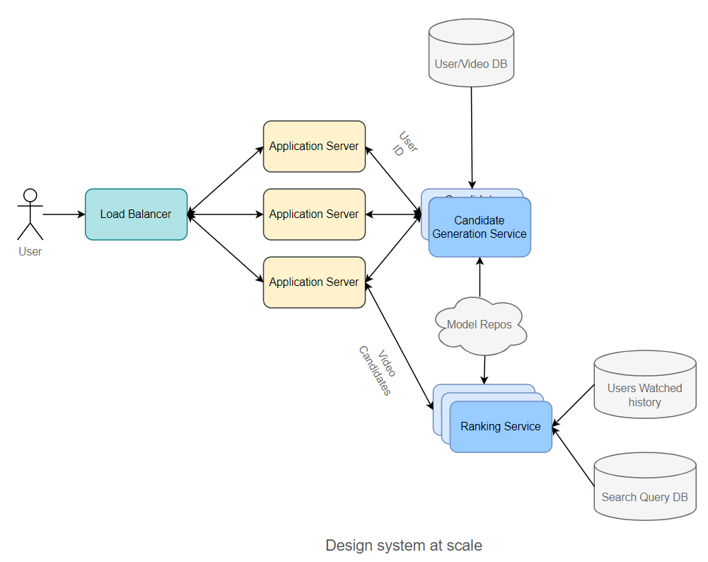
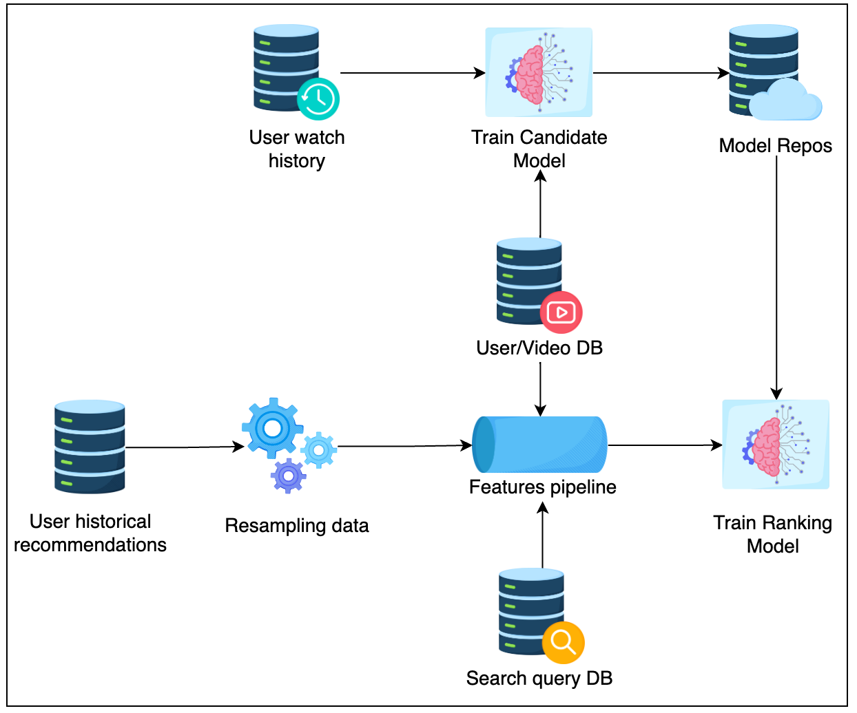
• Database
• Resampling data: Down-sampling negative samples;
• Feature pipeline: To provide high throughput, as we require this to retrain models multiple times, using Spark, Elastic MapReduce or Google DataProc;
• Model Repos: Store all models, using AWS S3 in general;
• Scale the design:
  • Kube-proxy could be used to enable the Candidate Generation Service to call Ranking Service directly, reducing latency even further;

During inference, one common pattern for the inference component is to frequently pull the latest models from Model Repos based on the timestamp, in order to get the latest model near real-time.

Follow-up

Q	A
How do we adapt to user behavior changing over time?	1.Read more about Multi-arm bandit 2.Use the Bayesian Logistic Regression Model so we can update prior data 3.Use different loss functions to be less sensitive with CTR

References ⭐

• Deep Neural Networks for YouTube Recommendations